I had originally planned to write about DeepSeek V4. Since it still hasn’t been released, I used the time to work on something that had been on my list for a while, namely, collecting, organizing, and refining the different LLM architectures I have covered over the past few years.

So, over the last two weeks, I turned that effort into an LLM architecture gallery (with 45 entries at the time of this writing), which combines material from earlier articles with several important architectures I had not documented yet. Each entry comes with a visual model card, and I plan to keep the gallery updated regularly.

You can find the gallery here: https://sebastianraschka.com/llm-architecture-gallery/

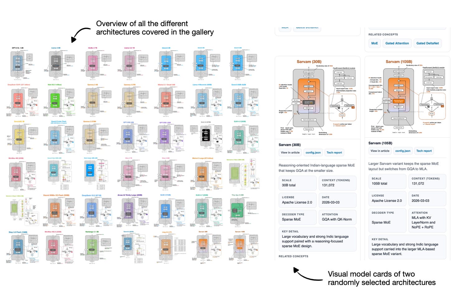
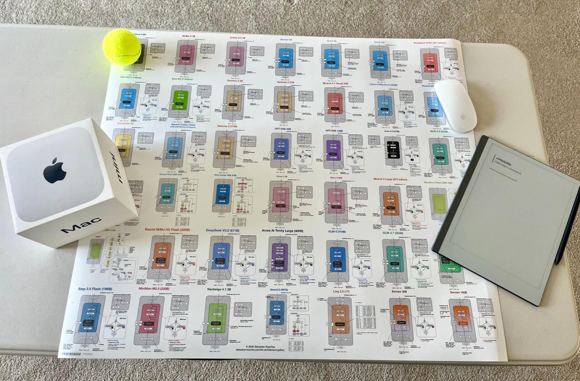
After I shared the initial version, a few readers also asked whether there would be a poster version. So, there is now a poster version via Redbubble. I ordered the Medium size (26.9 x 23.4 in) to check how it looks in print, and the result is sharp and clear. That said, some of the smallest text elements are already quite small at that size, so I would not recommend the smaller versions if you intend to have everything readable.

Alongside the gallery, I was/am also working on short explainers for a few core LLM concepts.

So, in this article, I thought it would be interesting to recap all the recent attention variants that have been developed and used in prominent open-weight architectures in recent years.

My goal is to make the collection useful both as a reference and as a lightweight learning resource. I hope you find it useful and educational!

1. Multi-Head Attention (MHA)

Self-attention lets each token look at the other visible tokens in the sequence, assign them weights, and use those weights to build a new context-aware representation of the input.

Multi-head attention (MHA) is the standard transformer version of that idea. It runs several self-attention heads in parallel with different learned projections, then combines their outputs into one richer representation.

The sections below start with a whirlwind tour of explaining self-attention to explain MHA. It’s more meant as a quick overview to set the stage for related attention concepts like grouped-query attention, sliding window attention, and so on. If you are interested in a longer, more detailed self-attention coverage, you might like my longer Understanding and Coding Self-Attention, Multi-Head Attention, Causal-Attention, and Cross-Attention in LLMs article.

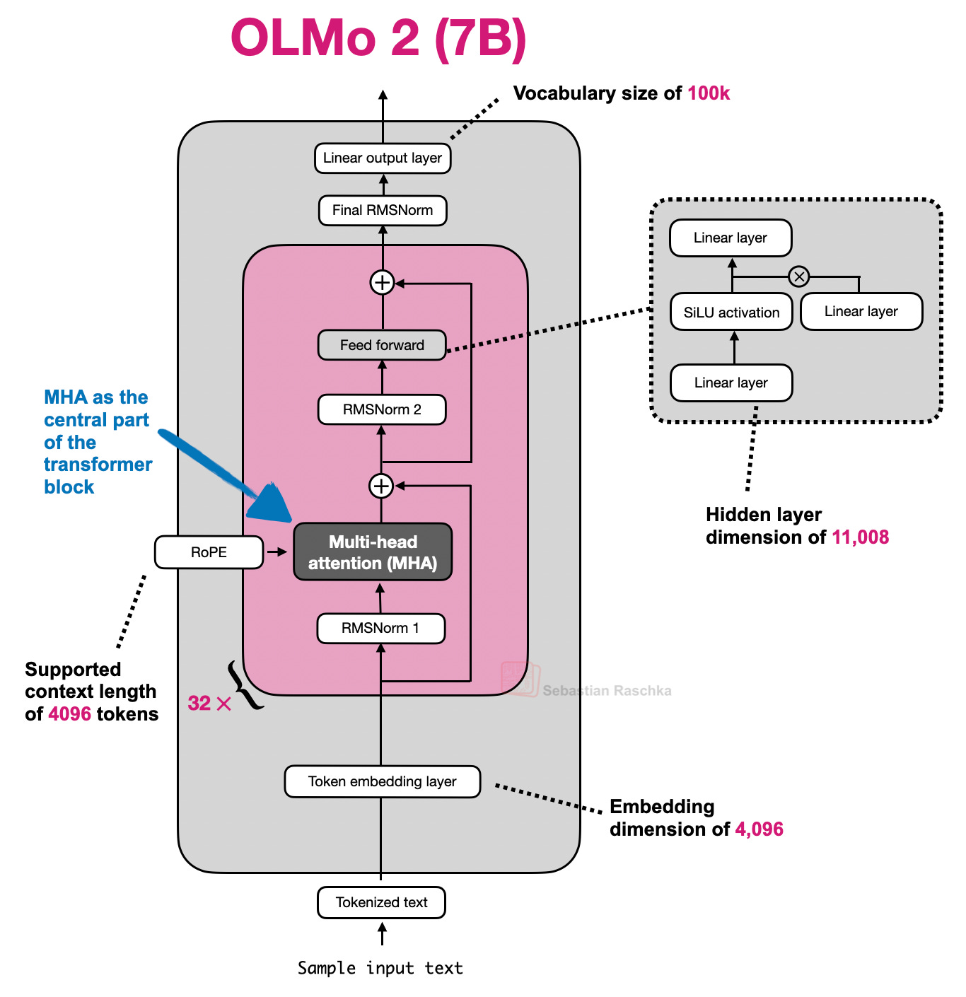
EXAMPLE ARCHITECTURES

GPT-2, OLMo 2 7B, and OLMo 3 7B

1.2 Historical Tidbits And Why Attention Was Invented

Attention predates transformers and MHA. Its immediate background is encoder-decoder RNNs for translation.

In those older systems, an encoder RNN would read the source sentence token by token and compress it into a sequence of hidden states, or in the simplest version into one final state. Then the decoder RNN had to generate the target sentence from that limited summary. This worked for short and simple cases, but it created an obvious bottleneck once the relevant information for the next output word lived somewhere else in the input sentence.

In short, the limitation is that the hidden state can’t store infinitely much information or context, and sometimes it would be useful to just refer back to the full input sequence.

The translation example below shows one of the limitations of this idea. For instance, a sentence can preserve many locally reasonable word choices and still fail as a translation when the model treats the problem too much like a word-by-word mapping. (The top panel shows an exaggerated example where we translate the sentence word by word; obviously, the grammar in the resulting sentence is wrong.) In reality, the correct next word depends on sentence-level structure and on which earlier source words matter at that step. Of course, this could still be translated fine with an RNN, but it would struggle with longer sequences or knowledge retrieval tasks because the hidden state can only store so much information as mentioned earlier.

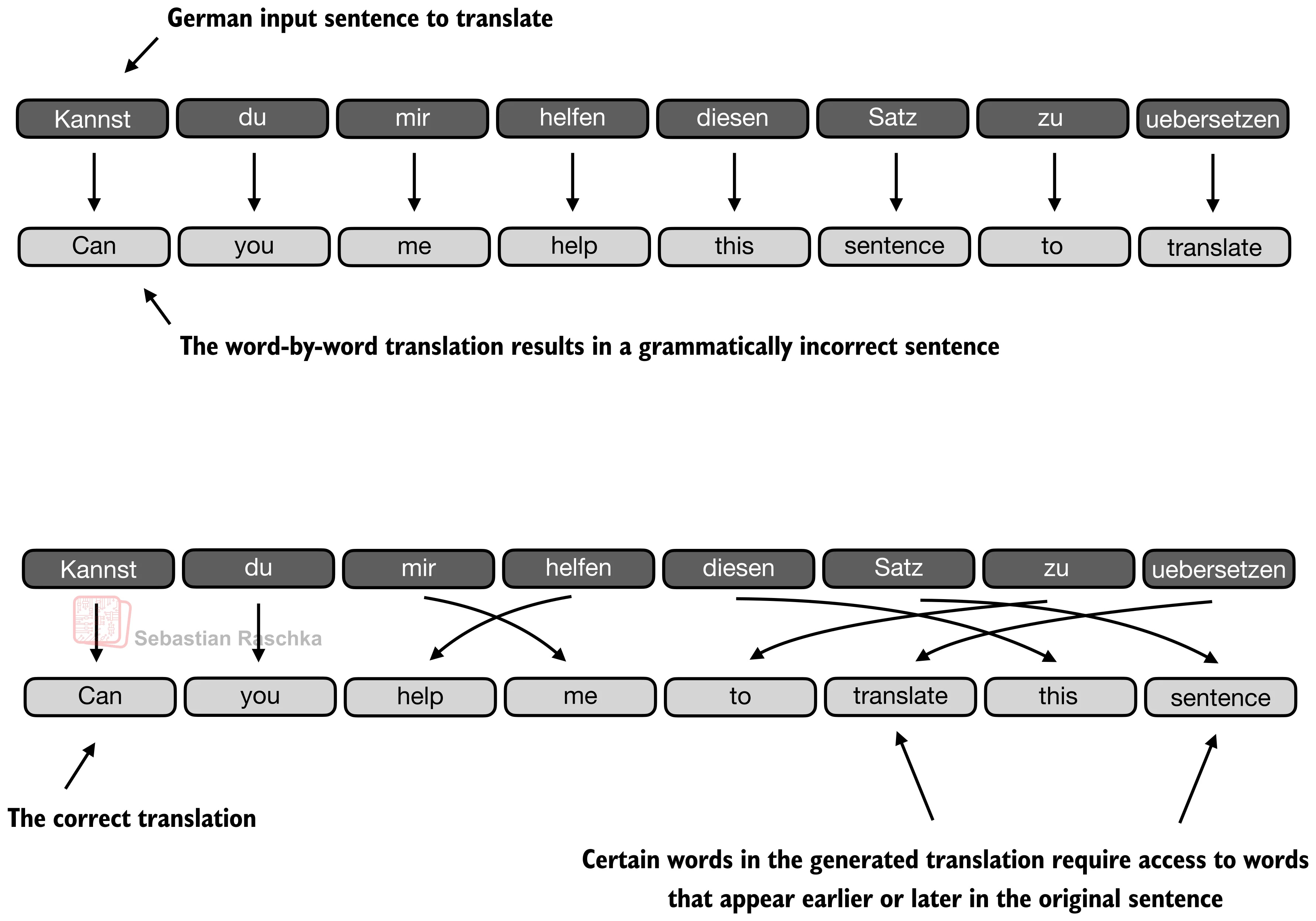
The next figure shows that change more directly. When the decoder is producing an output token, it should not be limited to one compressed memory path. It should be able to reach back to the more relevant input tokens directly.

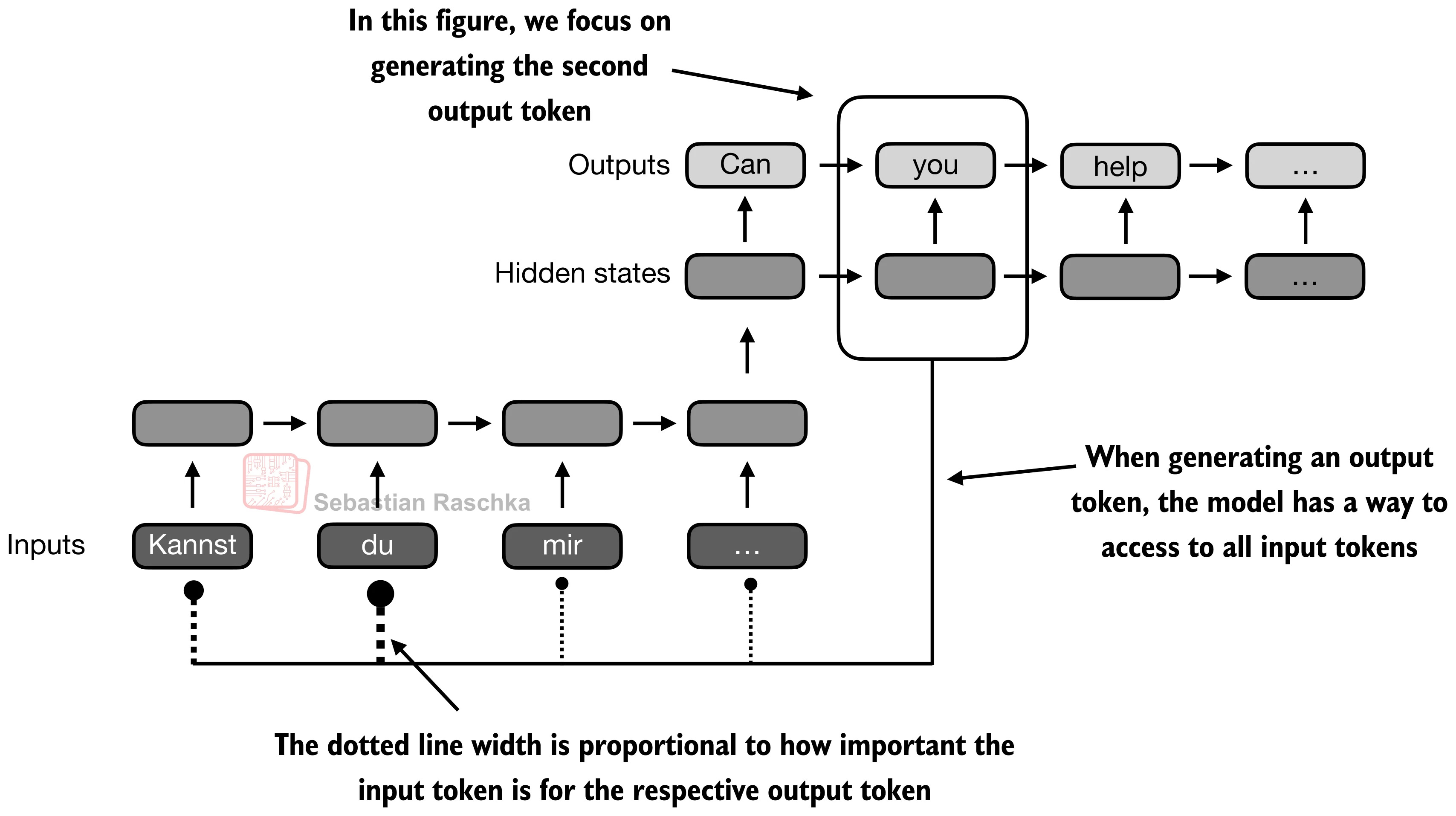
Transformers keep that core idea from the aforementioned attention-modified RNN but remove the recurrence. In the classic Attention Is All You Need paper, attention becomes the main sequence-processing mechanism itself (instead of being just part of an RNN encoder-decoder.)

In transformers, that mechanism is called self-attention, where each token in the sequence computes weights over all other tokens and uses them to mix information from those tokens into a new representation. Multi-head attention is the same mechanism run several times in parallel.

1.3 The Masked Attention Matrix

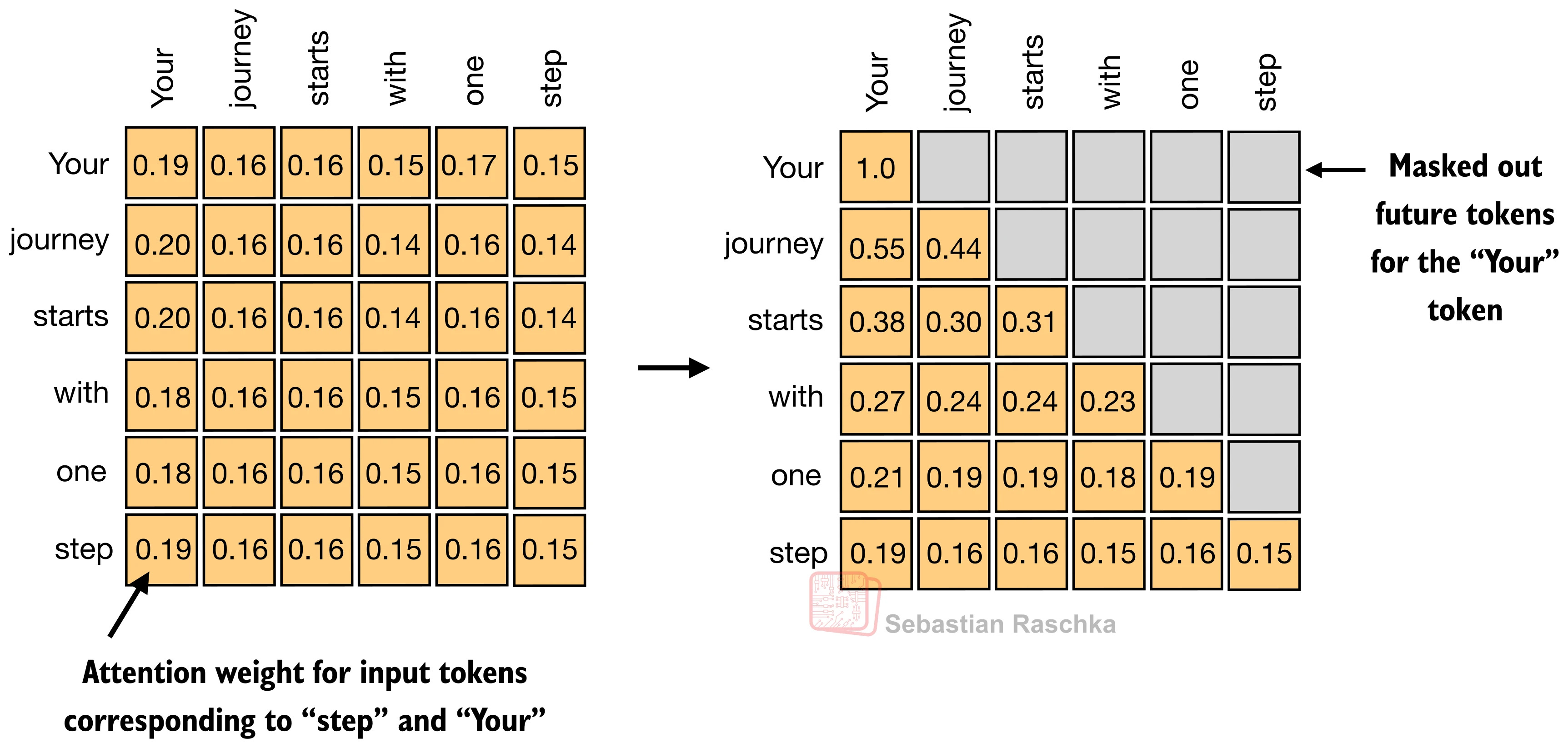
For a sequence of T tokens, attention needs one row of weights per token, so overall we get a T x T matrix.

Each row answers a simple question. When updating this token, how much should each visible token matter? In a decoder-only LLM, future positions are masked out, which is why the upper-right part of the matrix is grayed out in the figure below.

Self-attention is fundamentally about learning these token-to-token weight patterns, under a causal mask, and then using them to build context-aware token representations.

1.4 Self-Attention Internals

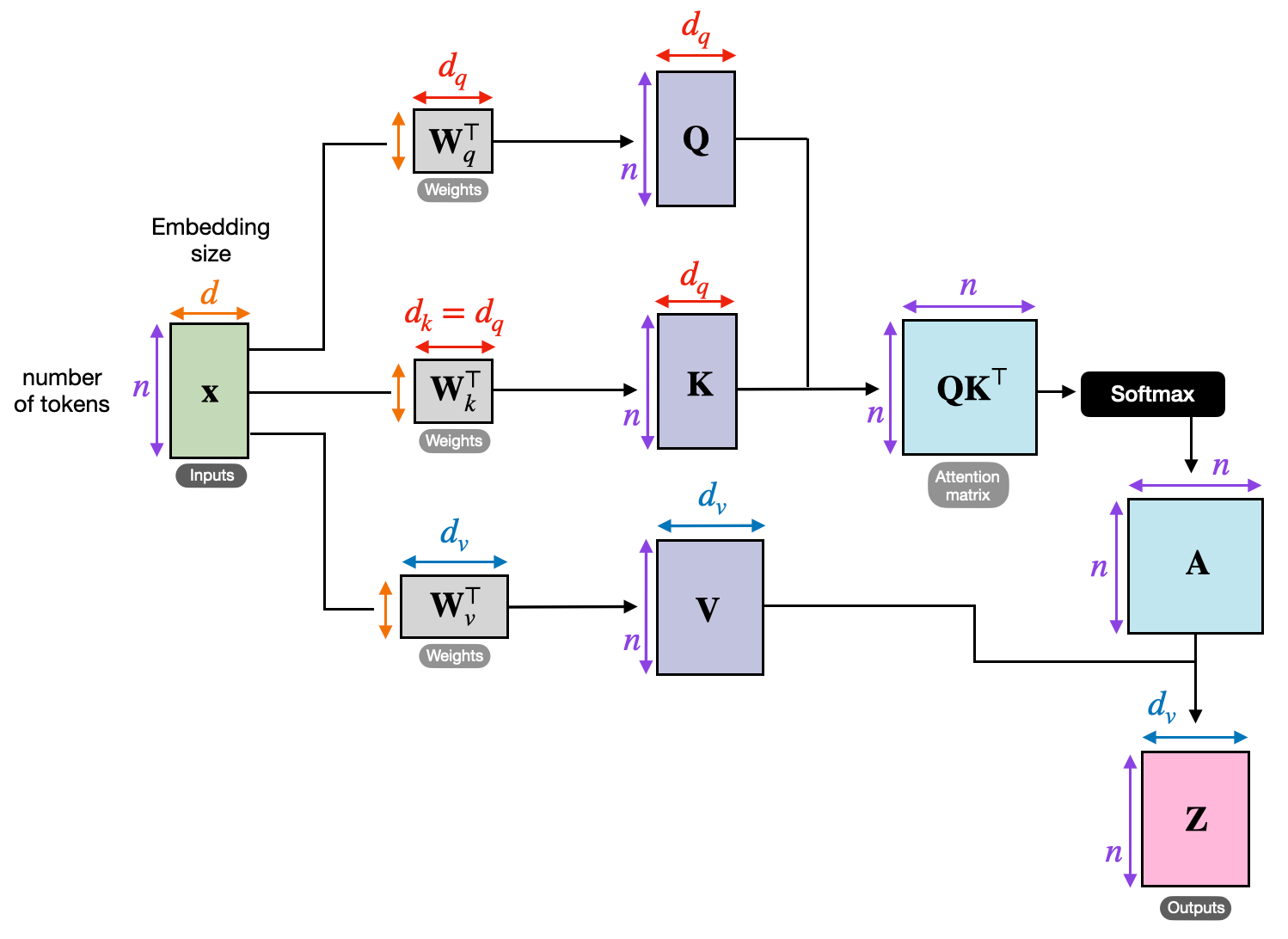
The next figure shows how the transformer computes the attention matrix (A) from the input embeddings X, which is then used to produce the transformed inputs (Z).

Here Q, K, and V stand for queries, keys, and values. The query for a token represents what that token is looking for, the key represents what each token makes available for matching, and the value represents the information that gets mixed into the output once the attention weights have been computed.

The steps are as follows:

• Wq, Wk, and Wv are weight matrices that project the input embeddings into Q, K, and V

• QK^T produces the raw token-to-token relevance scores

• softmax converts those scores into the normalized attention matrix A that we discussed in the previous section

• A is applied to V to produce the output matrix Z

Note that the attention matrix is not a separate hand-written object. It emerges from Q, K, and softmax.

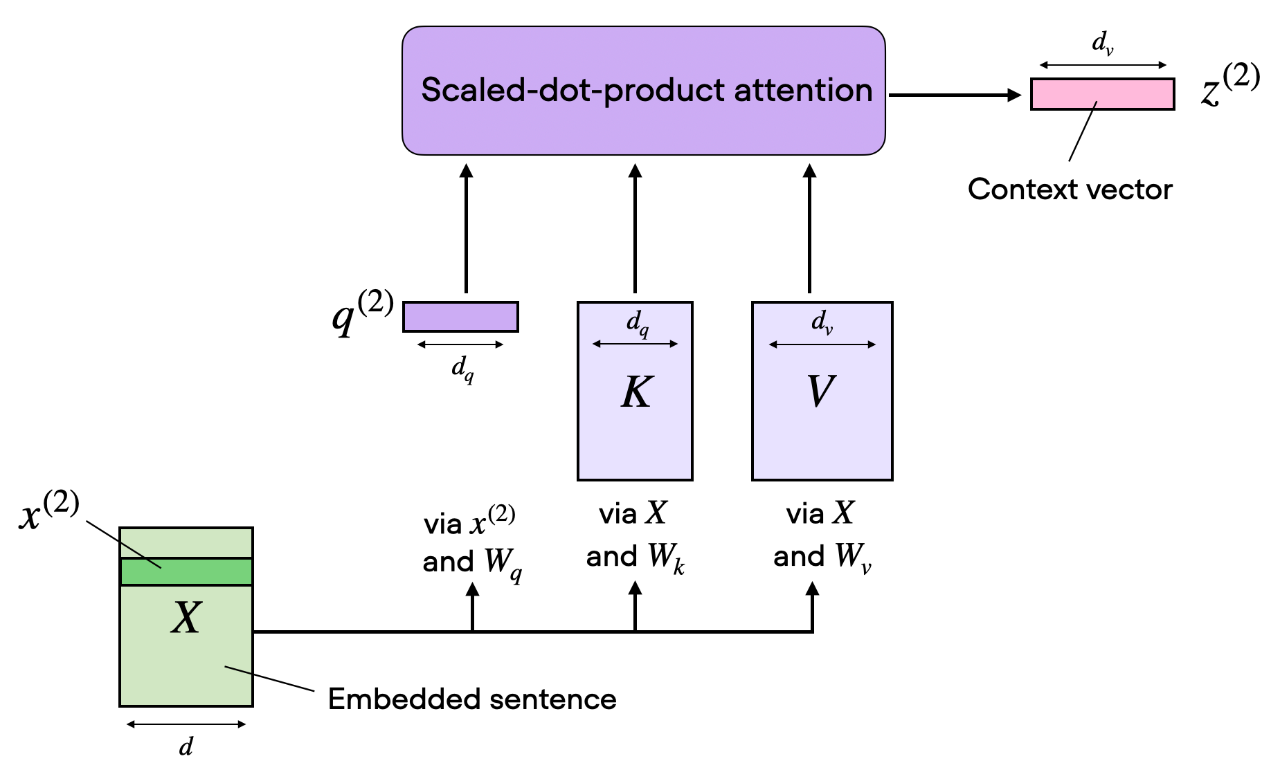
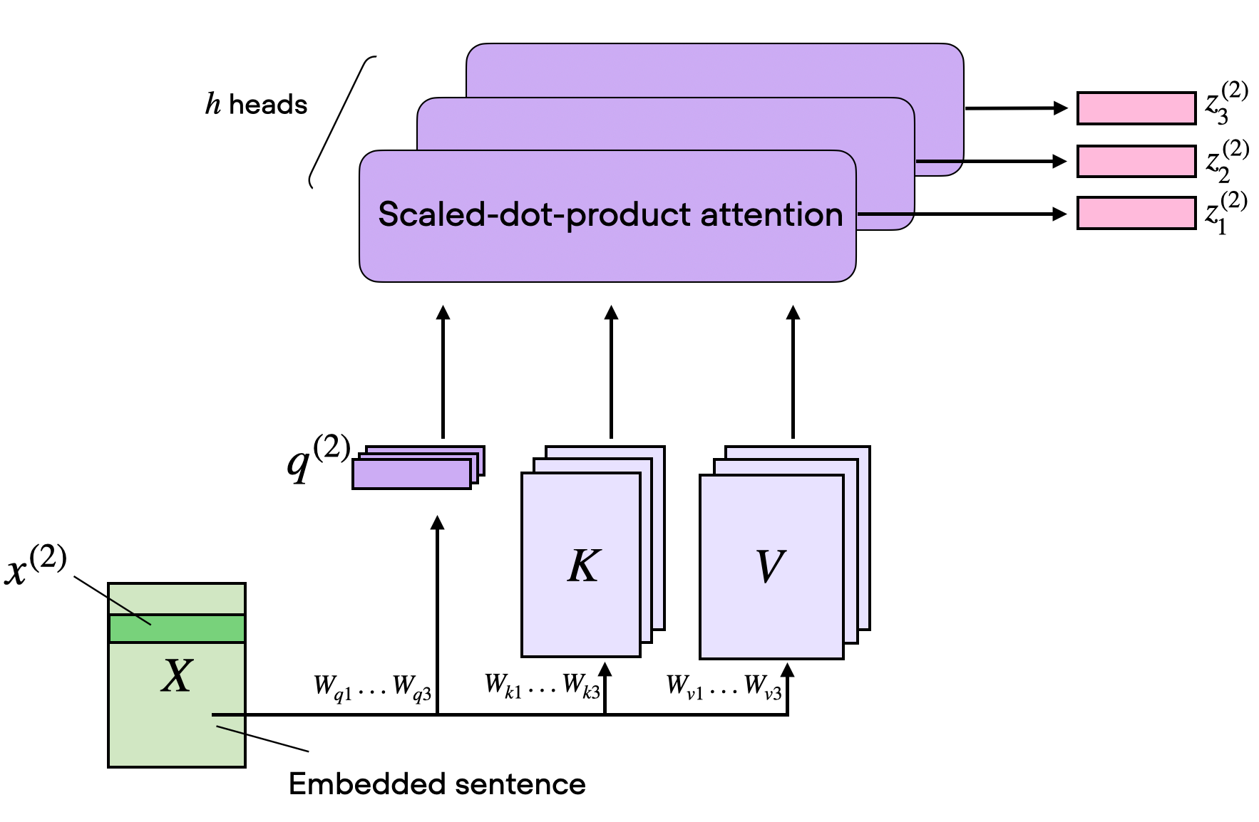
The next figure shows the same concept as the previous figure but the attention matrix computation is hidden inside the “scaled-dot-product attention” box, and we perform the computation only for one input token instead of all input tokens. This is to show a compact form of self-attention with a single head before extending this to multi-head attention in the next section.

1.5 From One Head To Multi-Head Attention

One set of Wq/Wk/Wv matrices gives us one attention head, which means one attention matrix and one output matrix Z. (This concept was illustrated in the previous section.)

Multi-head attention simply runs several of these heads in parallel with different learned projection matrices.

This is useful because different heads can specialize in different token relationships. One head might focus on short local dependencies, another on broader semantic links, and another on positional or syntactic structure.

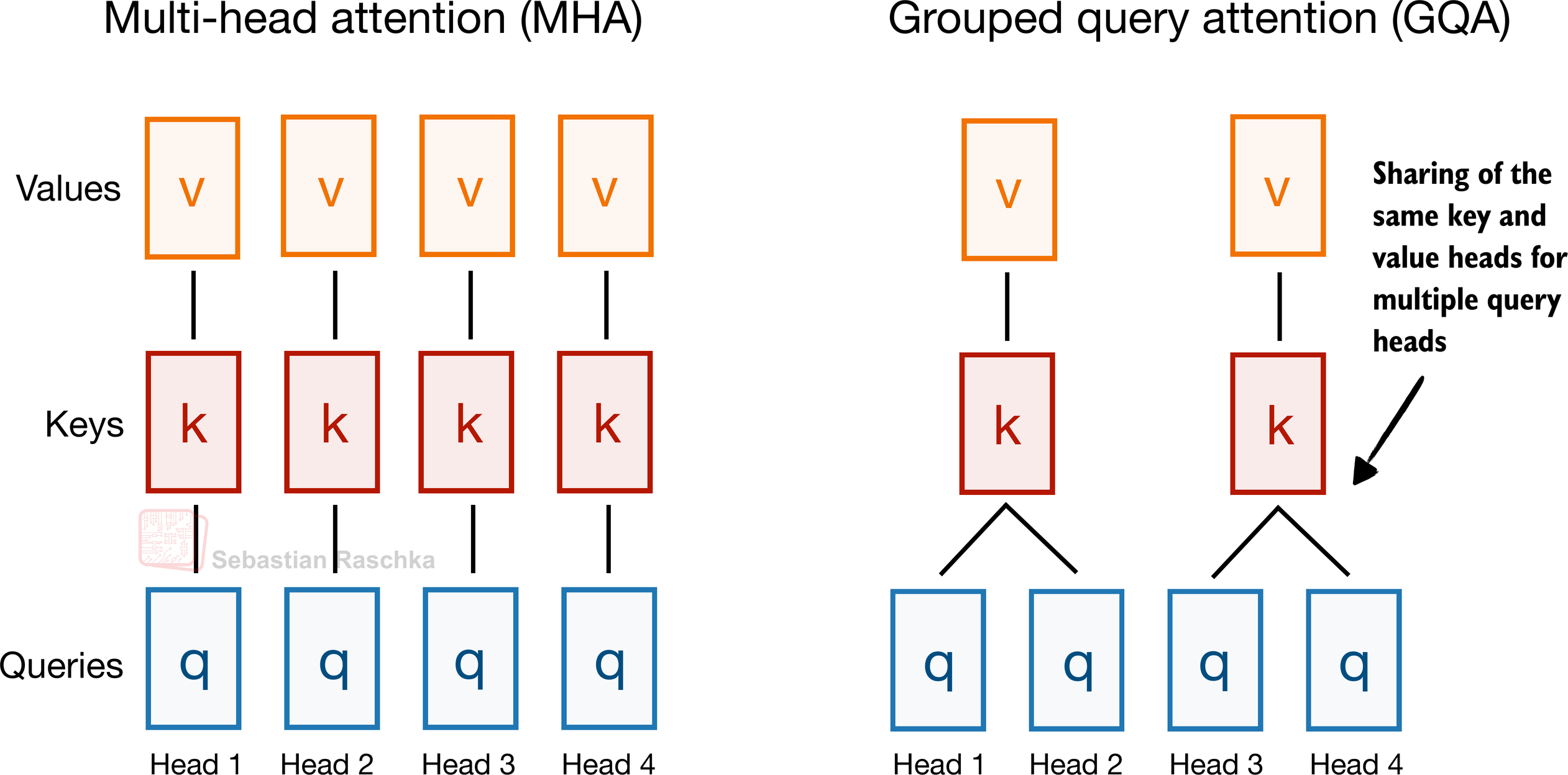
2. Grouped-Query Attention (GQA)

Grouped-query attention is an attention variant derived from standard MHA. It was introduced in the 2023 paper GQA: Training Generalized Multi-Query Transformer Models from Multi-Head Checkpoints by Joshua Ainslie and colleagues.

Instead of giving every query head its own keys and values, it lets several query heads share the same key-value projections, which makes KV caching much cheaper (primarily as a memory reduction) without changing the overall decoder recipe very much.

EXAMPLE ARCHITECTURES

Dense: Llama 3 8B, Qwen3 4B, Gemma 3 27B, Mistral Small 3.1 24B, SmolLM3 3B, and Tiny Aya 3.35B.
Sparse (Mixture-of-Experts): Llama 4 Maverick, Qwen3 235B-A22B, Step 3.5 Flash 196B, and Sarvam 30B.

2.1 Why GQA Became Popular

In my architecture comparison article, I framed GQA as the new standard replacement for classic multi-head attention (MHA). The reason is that standard MHA gives every head its own keys and values, which is more optimal from a modeling perspective but expensive once we have to keep all of that state in the KV cache during inference.

In GQA, we keep a larger set of query heads, but we reduce the number of key-value heads and let multiple queries share them. That lowers both parameter count and KV-cache traffic without making drastic implementation changes like multi-head latent attention (MLA), which will be discussed later.

In practice, that made and keeps it a very popular choice for labs that wanted something cheaper than MHA but simpler to implement than newer compression-heavy alternatives like MLA.

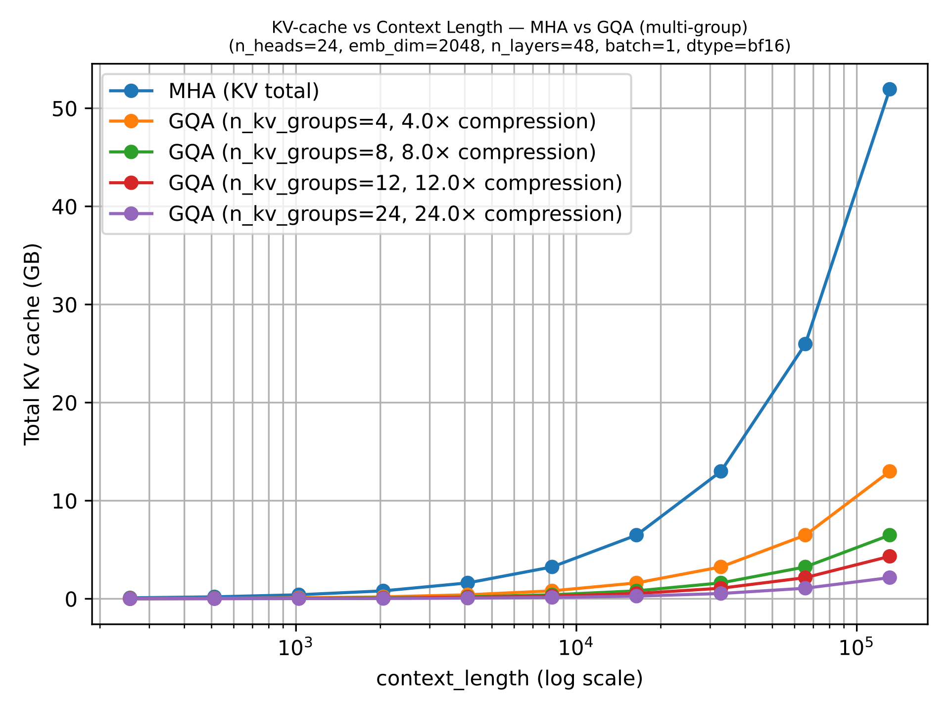
2.2 GQA Memory Savings

GQA results in big savings in KV storage, since the fewer key-value heads we keep per layer, the less cached state we need per token. That is why GQA becomes more useful as sequence length grows.

GQA is also a spectrum. If we reduce all the way down to one shared K/V group, we are effectively in multi-query attention territory, which is even cheaper but can hurt modeling quality more noticeably. The sweet spot is usually somewhere in between multi-query attention (1 shared group) and MHA (where K/V groups are equal to the number of queries), where the cache savings are large but the modeling degradation relative to MHA stays modest.

2.3 Why GQA Still Matters In 2026

More advanced variants such as MLA are becoming popular because they can offer better modeling performance at the same KV efficiency levels (e.g., as discussed in the ablation studies of the DeepSeek-V2 paper), but they also involve a more complicated implementation and a more complicated attention stack.

GQA remains appealing because it is robust, easier to implement, and also easier to train (since there are fewer hyperparameter tunings necessary, based on my experience).

That is why some of the newer releases still stay deliberately classic here. E.g., in my Spring Architectures article, I mentioned that MiniMax M2.5 and Nanbeige 4.1 as models that remained very classic, using only grouped-query attention without piling on other efficiency tricks. Sarvam is a particularly useful comparison point as well: the 30B model keeps classic GQA, while the 105B version switches to MLA.

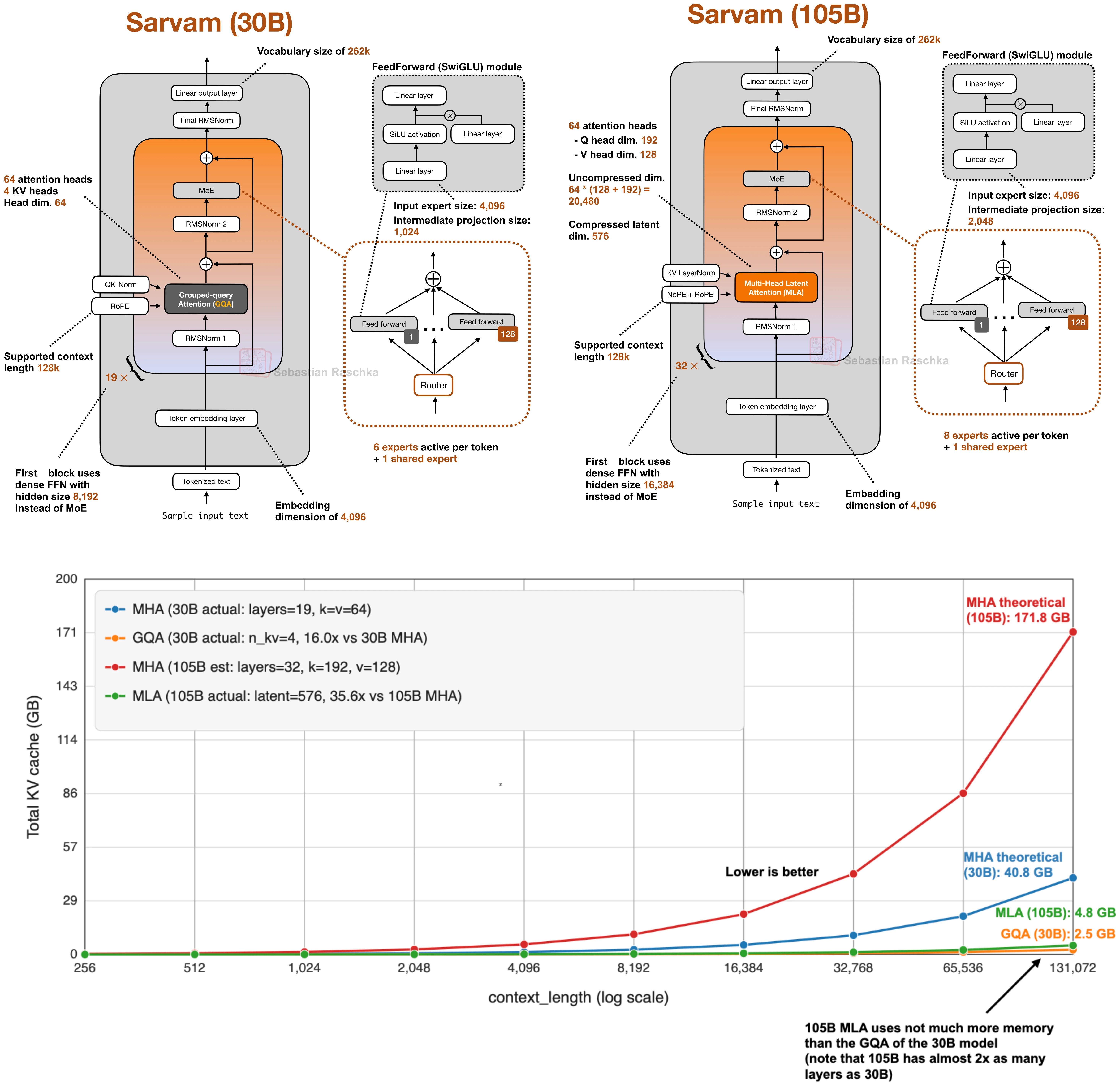
3. Multi-Head Latent Attention (MLA)

The motivation behind Multi-head Latent Attention (MLA) is similar to Grouped-Query Attention (GQA). Both are solutions for reducing KV-cache memory requirements. The difference between GQA and MLA is that MLA shrinks the cache by compressing what gets stored rather than by reducing how many K/Vs are stored by sharing heads.

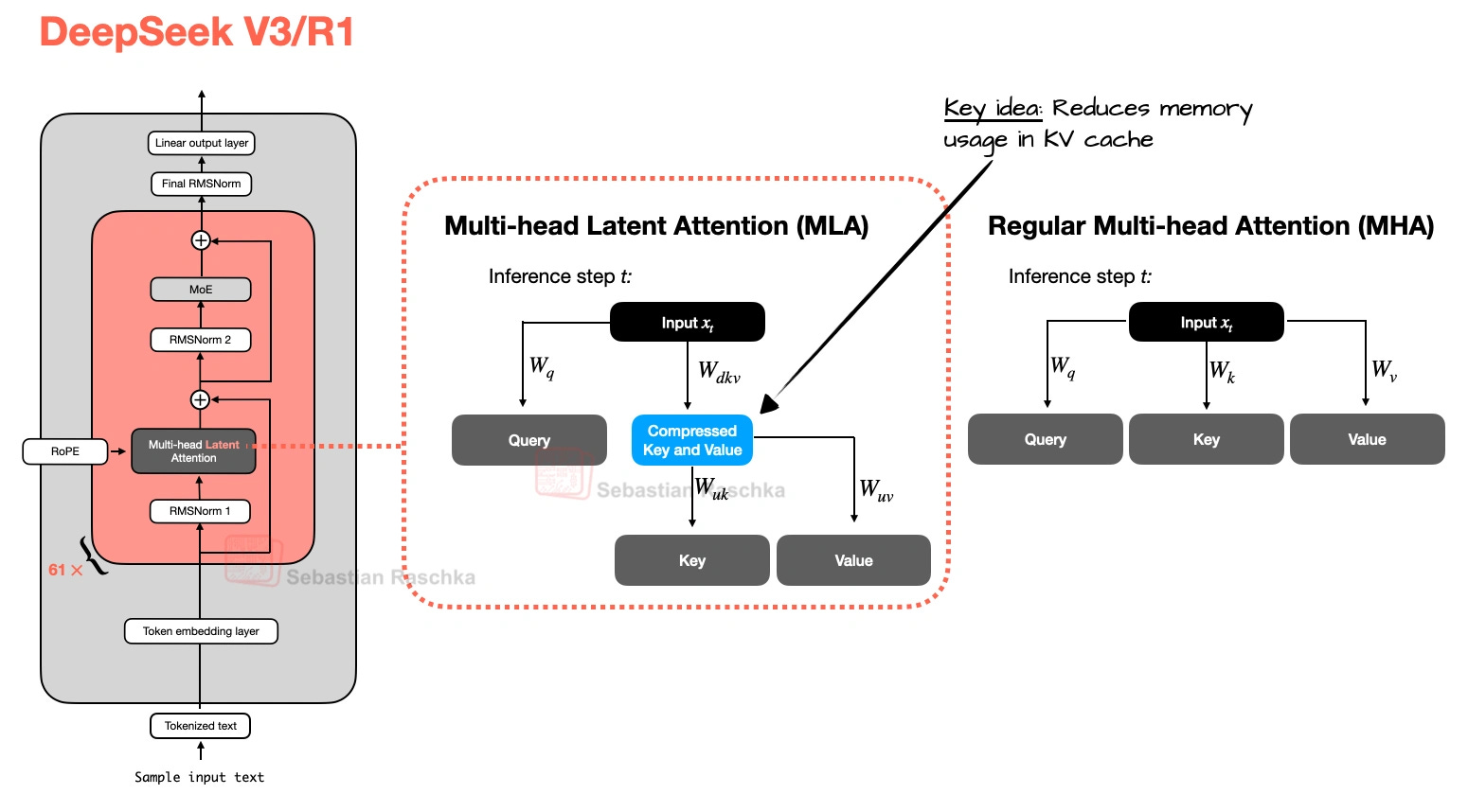
MLA, originally proposed in the